This post is based on two papers:
- A. Luthra, T. Yang, T. Galanti. “Self-Supervised Contrastive Learning is Approximately Supervised Contrastive Learning”, NeurIPS 2025.
- A. Luthra, T. Yang, T. Galanti. “On the Alignment Between Supervised and Self-Supervised Contrastive Learning”, ICLR 2025.
Introduction
Self-supervised contrastive learning trains on unlabeled data, yet the learned features often look remarkably semantic: same-class samples cluster together, linear probes perform well, and downstream transfer can approach supervised pre-training. That raises a basic question: how can a method that never sees labels learn representations that look so class-aware?
In this post, we argue that contrastive learning is much closer to supervised contrastive learning than its name suggests. This closeness operates at two levels, each addressed by one of the papers above.
Part I: The losses are close
The setup
Consider a labeled dataset $S = {(x_i,y_i)}_{i=1}^N$, but assume that during self-supervised training we only use the inputs $x_i$, not the labels $y_i$. For each sample $x_i$, we generate $K$ augmentations and map them through an encoder $f$: $z_i^l = f(\alpha_l(x_i))$.
A standard decoupled contrastive loss (DCL) takes the form
\[\mathcal{L}^{\mathrm{DCL}}(f) = -\frac{1}{K^2N}\sum_{l_1,l_2=1}^K\sum_{i=1}^N \log\left(\frac{\exp(\mathrm{sim}(z_i^{l_1},z_i^{l_2}))}{\sum_{l_3=1}^K\sum_{j\neq i}\exp(\mathrm{sim}(z_i^{l_1},z_j^{l_3}))}\right).\]This is a purely self-supervised objective. It rewards two views of the same sample for being similar and penalizes similarity to all other samples.
Now compare it with a supervised variant that excludes same-class negatives from the denominator:
\[\mathcal{L}^{\mathrm{NSCL}}(f) = -\frac{1}{K^2N}\sum_{l_1,l_2=1}^K\sum_{i=1}^N \log\left(\frac{\exp(\mathrm{sim}(z_i^{l_1},z_i^{l_2}))}{\sum_{l_3=1}^K\sum_{j:y_j\neq y_i}\exp(\mathrm{sim}(z_i^{l_1},z_j^{l_3}))}\right).\]We call this NSCL, for negatives-only supervised contrastive learning. The two losses differ in exactly one place: DCL treats every other sample as a negative, while NSCL removes same-class samples from the denominator.
Why the gap is small
Suppose the dataset is balanced, with $C$ classes and $n$ samples per class, so $N = Cn$. Fix an anchor. In DCL, the denominator sums over all $N-1$ other samples. In NSCL, it sums over only the $N-n = n(C-1)$ different-class samples. The same-class terms that appear in DCL but not in NSCL number exactly $n-1$, a fraction roughly $1/C$ of the total. So when $C$ is large, the two denominators are nearly the same.
This can be made precise:
The bound is both label-agnostic and architecture-independent: it holds for any encoder $f$, without assumptions on the data distribution or the model class. The gap shrinks as $O(1/C)$, which means that for problems with many semantic classes, DCL is already almost NSCL.
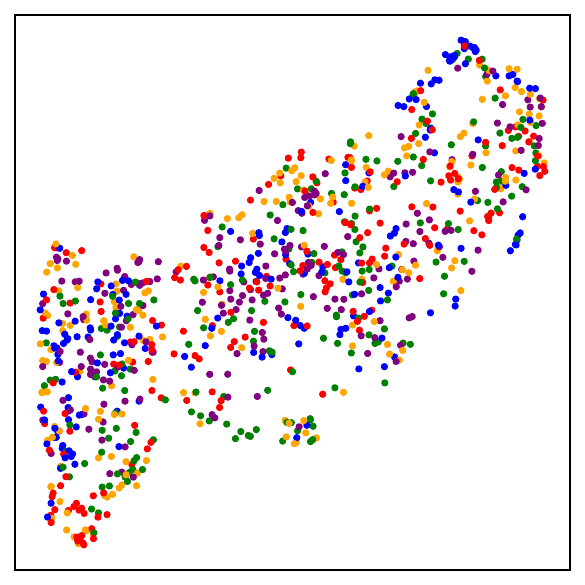
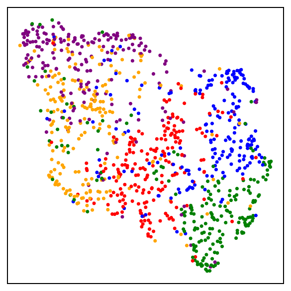
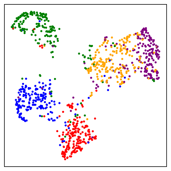
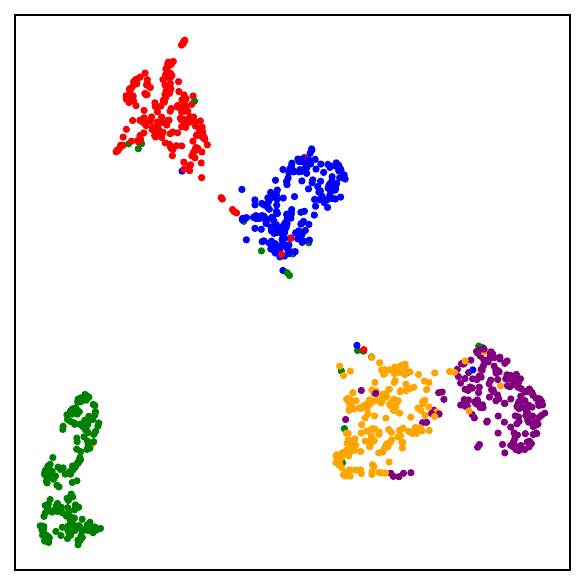
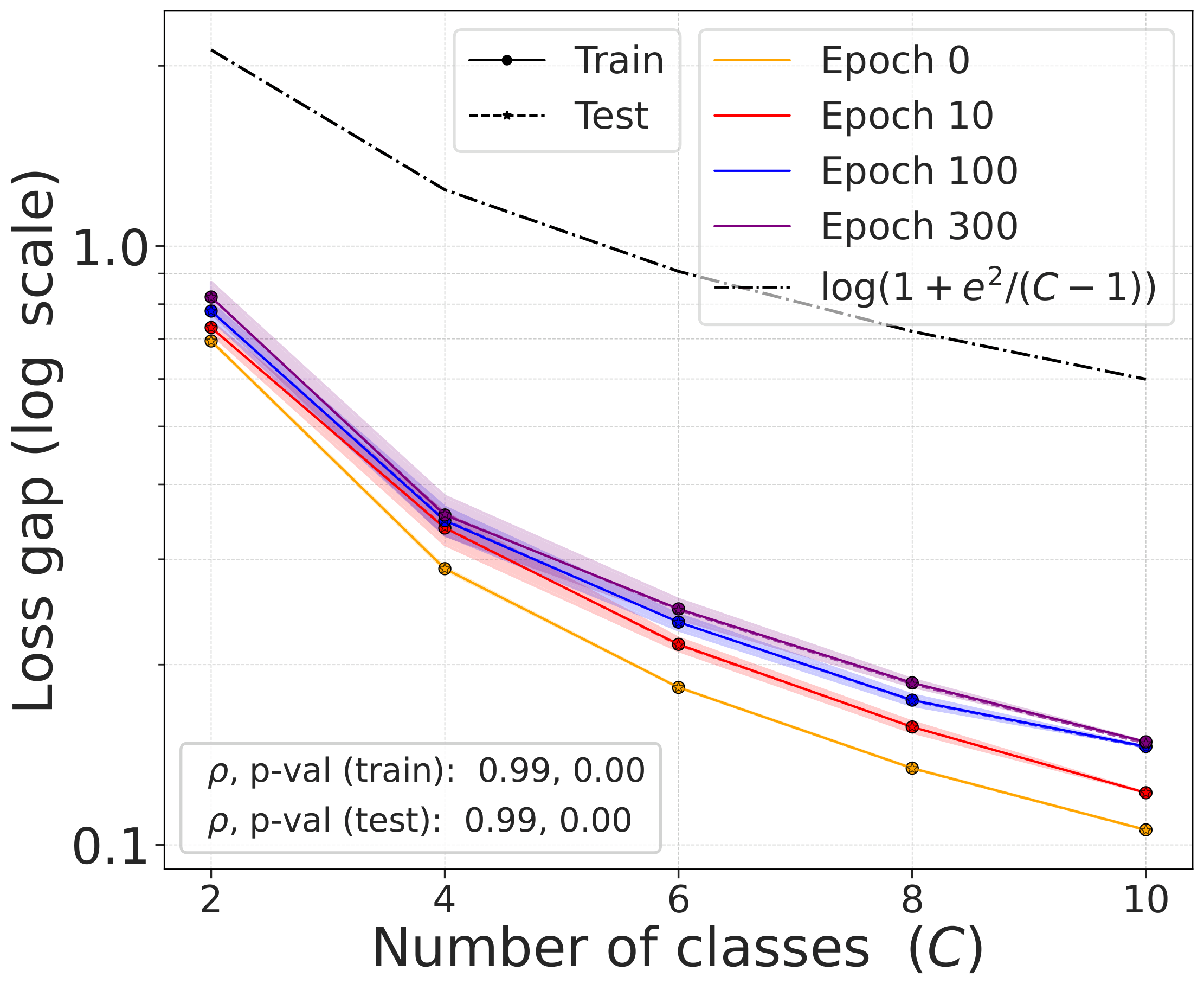
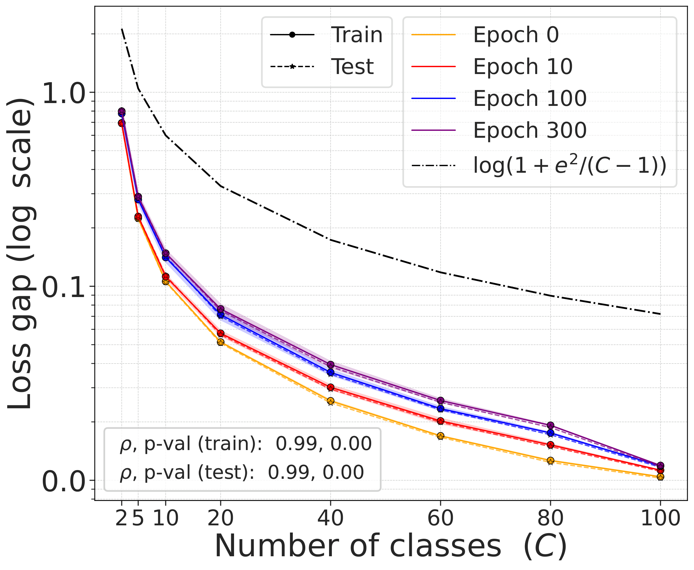
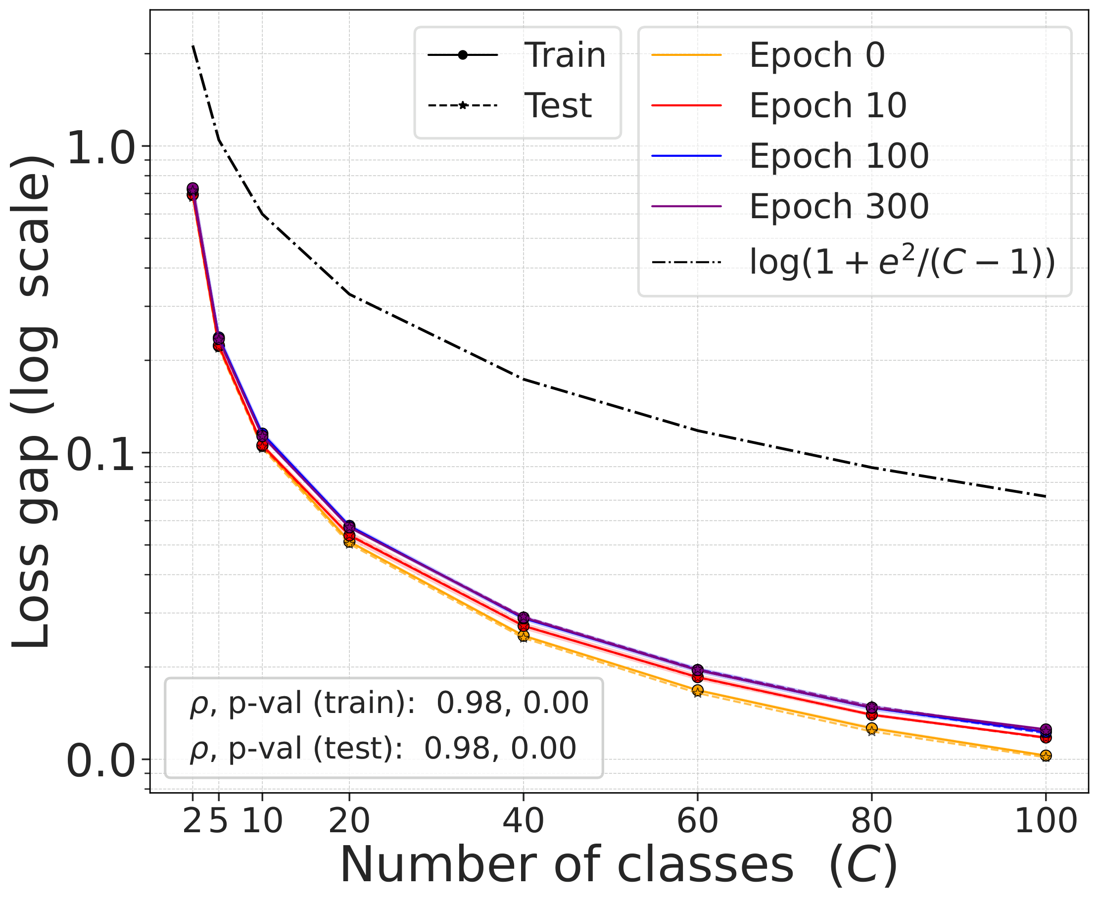
Validating the bound during training
We train models using SimCLR to minimize the DCL loss and track both losses throughout training, along with the theoretical upper bound $\mathcal{L}^{\mathrm{NSCL}}(f) + \log(1+\tfrac{n_{\max}\mathrm{e}^2}{N-n_{\max}})$.
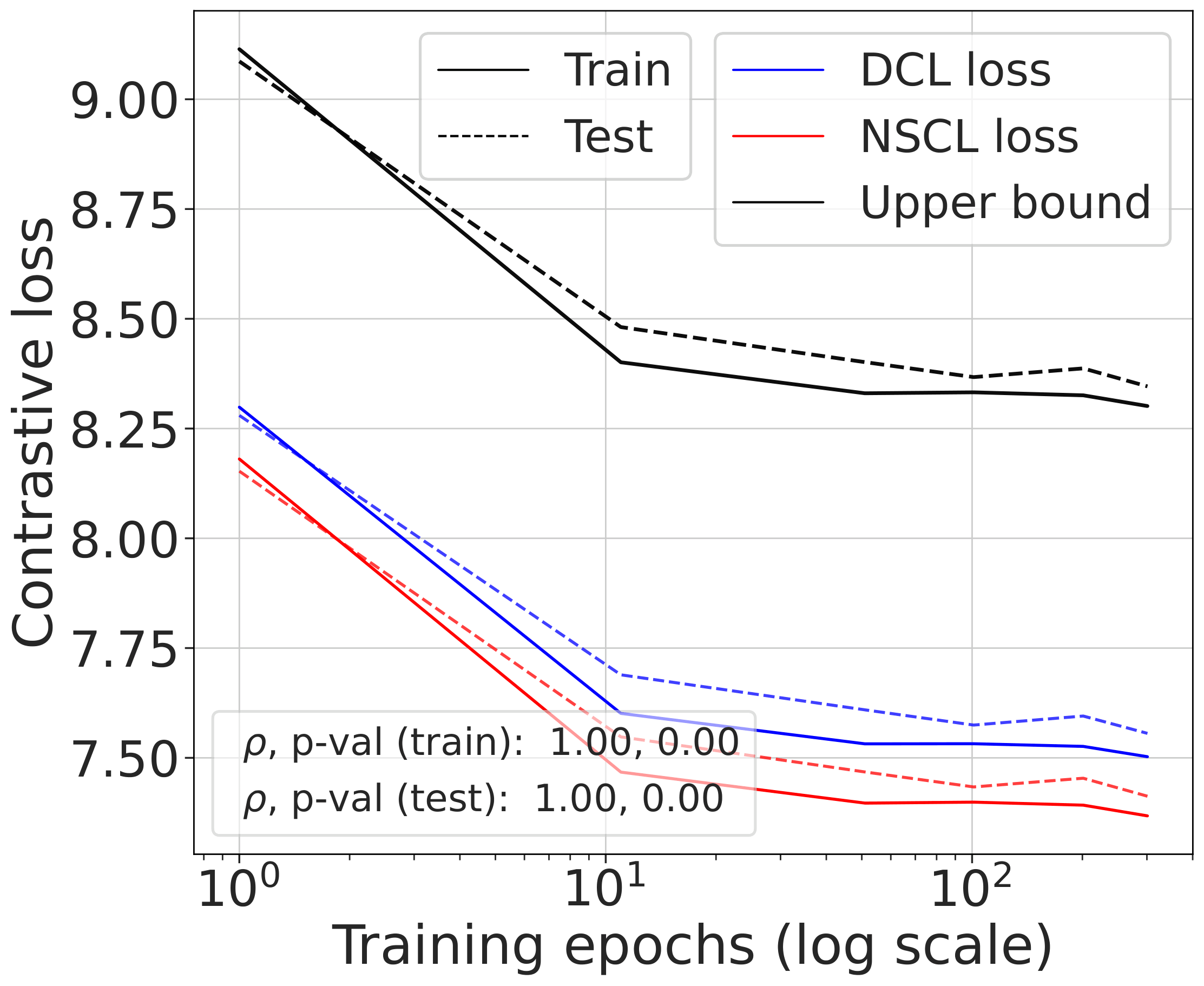
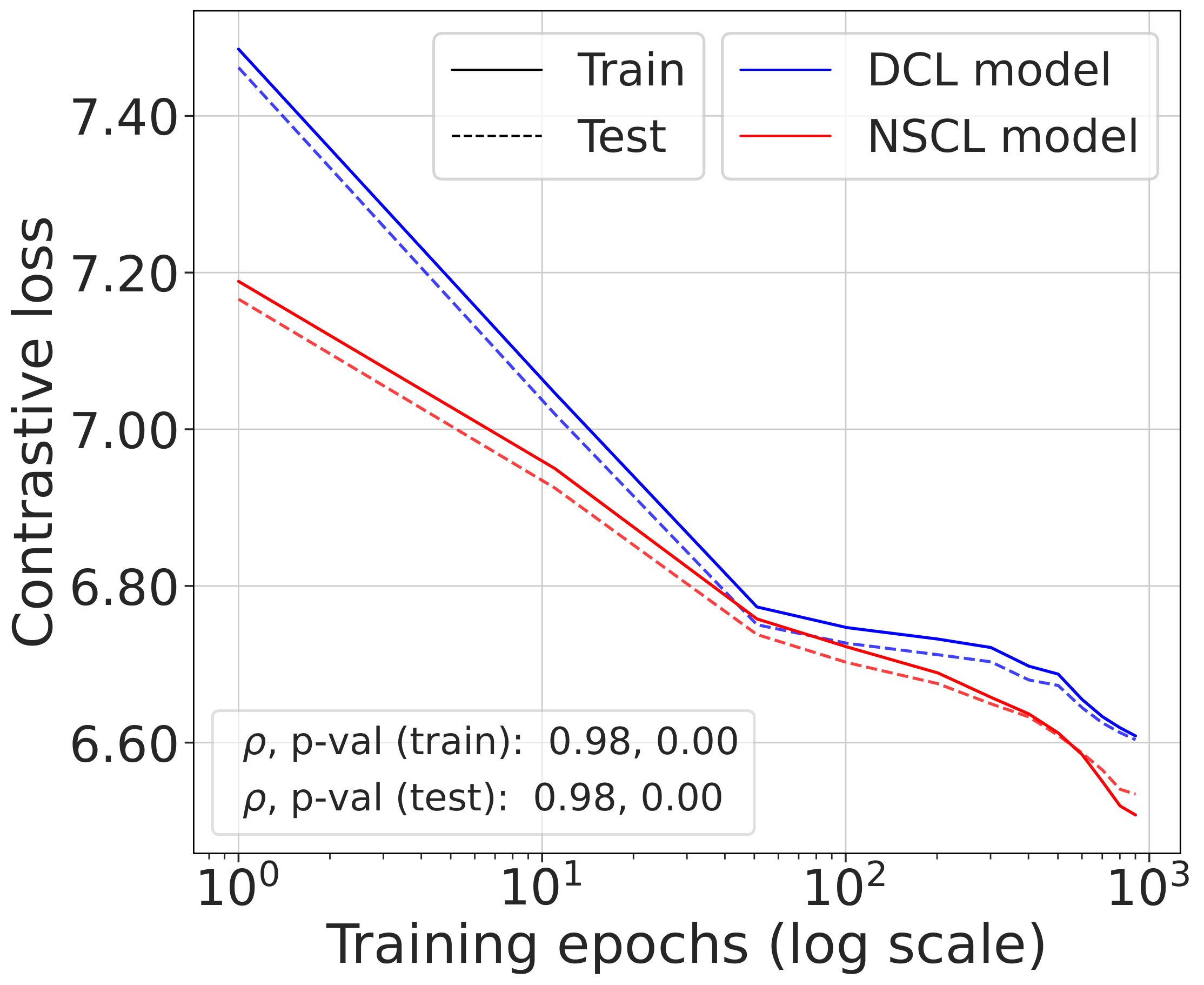
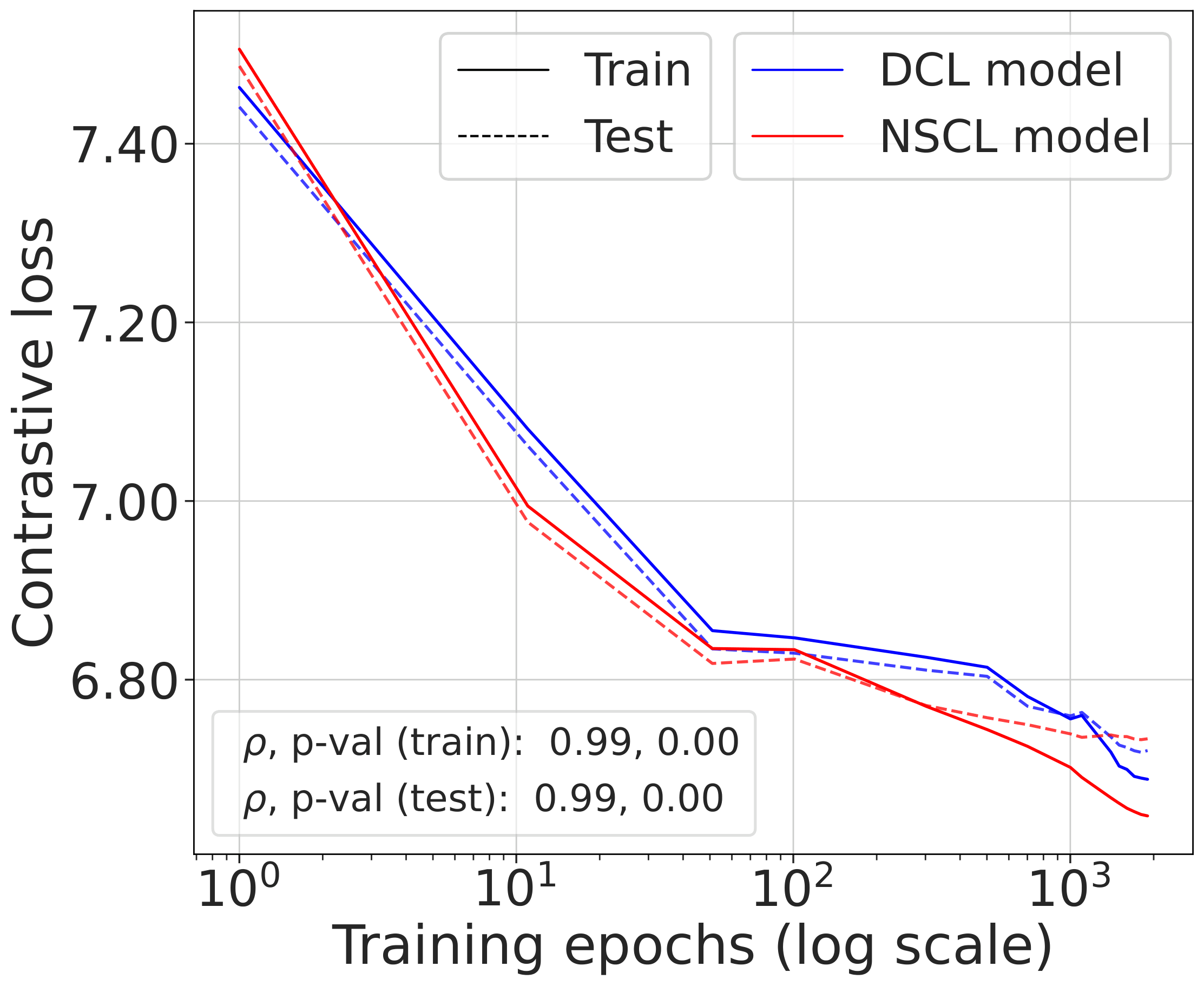
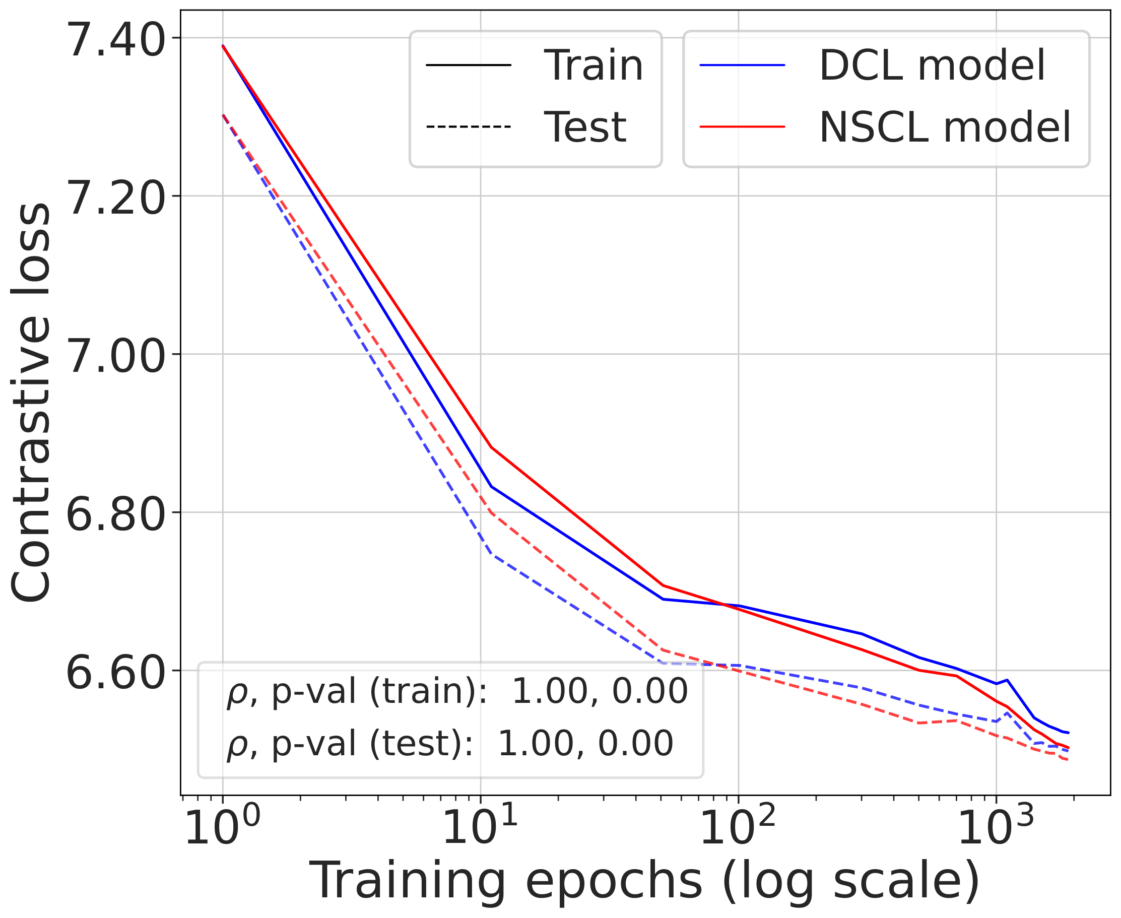
The DCL loss consistently upper bounds the NSCL loss, and the two become closer for tasks with more classes. When $C$ is large, for example $C=100$, the bound is very tight. Moreover, the NSCL losses of DCL-trained and NSCL-trained models are comparable at convergence, indicating that optimizing DCL leads to representations that are similarly clustered.
The gap scales as predicted with $C$
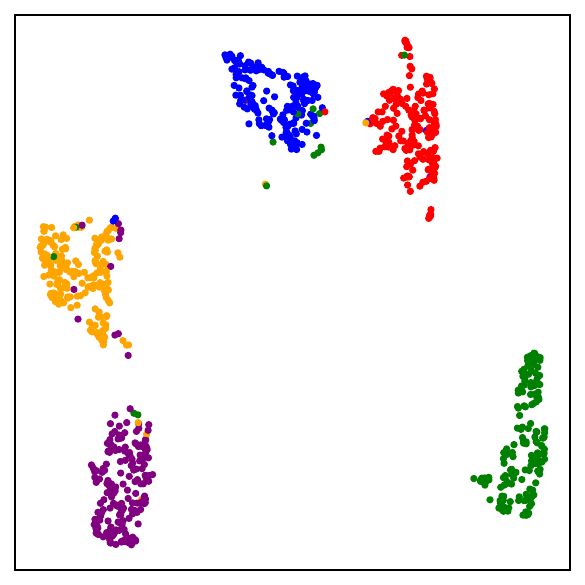
What NSCL minimizers look like
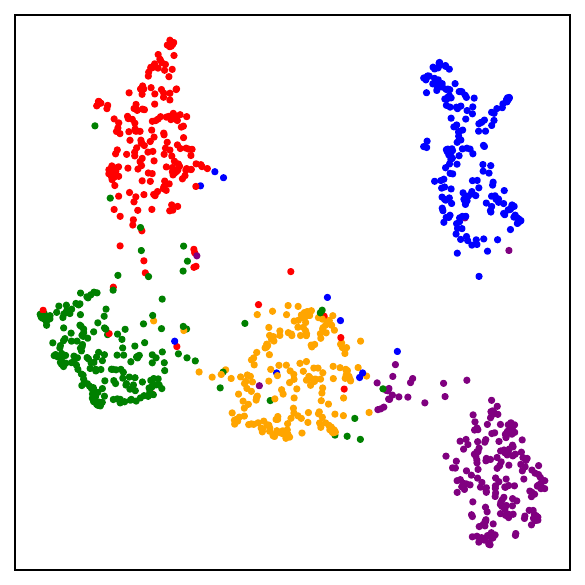
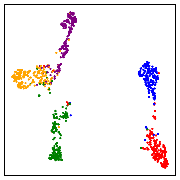
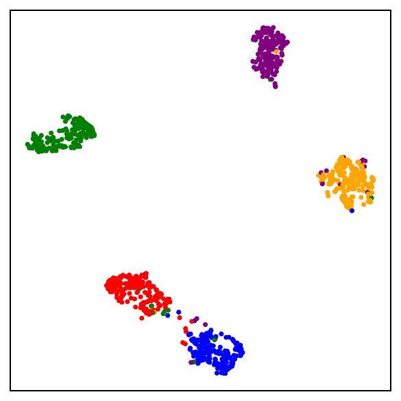
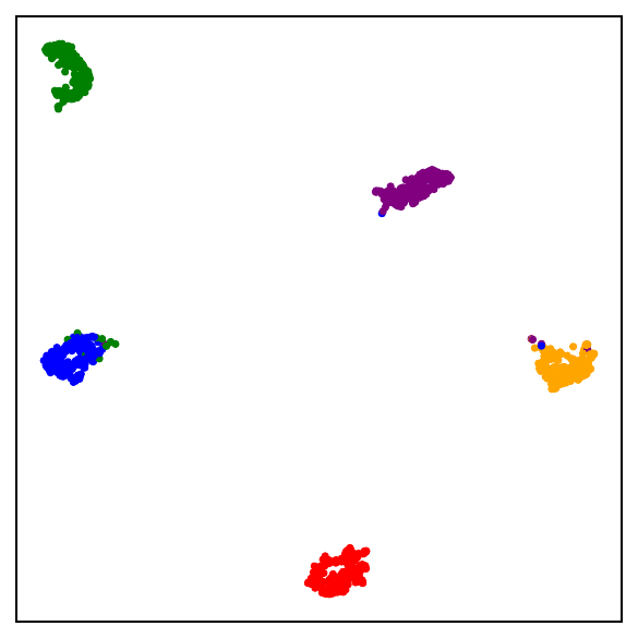
Beyond simply being a supervised loss, NSCL gives us a tractable bridge for understanding the geometry induced by contrastive learning. This raises a natural question: what kind of representations are learned by minimizing NSCL? Since NSCL serves as the supervised counterpart of DCL, understanding its global minimizers helps reveal the structure that self-supervised contrastive learning is implicitly approaching. In particular, any global minimizer of the NSCL loss exhibits three striking properties:
- Augmentation collapse: all augmented views of the same sample map to the same point.
- Within-class collapse: all samples from the same class share a single representation.
- Simplex ETF structure: the resulting class centers form a simplex equiangular tight frame, a maximally separated, symmetric configuration on the unit sphere.
Part II: The representations are close
Loss-level closeness is useful, but it does not by itself imply similar learned geometry. A small objective gap could still drive optimization in different directions. The second paper addresses this directly.
Shared-randomness coupling
Consider training CL and NSCL under shared randomness: same initialization, same mini-batches, same augmentations. The only difference between the two runs is the objective.
To compare the learned representations, define the cosine similarity matrix
\[\Sigma(Z)_{ij} = \cos(z_i,z_j),\]which captures the geometry of the representation directly. From it, standard alignment metrics follow: CKA (centered kernel alignment) and RSA (representational similarity analysis).
The similarity matrices stay close
Under the coupled training protocol, the difference between the CL and NSCL similarity matrices throughout training satisfies a bound of the form
\[\|\Sigma_T^{\mathrm{CL}}-\Sigma_T^{\mathrm{NS}}\|_F \lesssim \frac{e^{2/\tau}}{\tau C \sqrt{B}} \cdot \exp\left(\frac{1}{2\tau^2 B}\sum_{t=0}^{T-1}\eta_t\right)\cdot \left(\sum_{t=0}^{T-1}\eta_t\right).\]The right-hand side gets smaller when the number of classes $C$ is larger, the batch size $B$ is larger, the temperature $\tau$ is higher, and the cumulative step size $\sum_{t=0}^{T-1}\eta_t$ is more moderate. The same regimes that make the loss gap small also keep the representations aligned.
This immediately yields lower bounds on CKA and RSA:
where $\rho_T$ and $r_T$ are normalized versions of the similarity-matrix discrepancy.
Empirical confirmation: RSA and CKA are consistently high
The theoretical bounds predict that representation geometry should remain aligned even as parameters diverge. To test this directly, we train DCL and NSCL models under exactly matched conditions, same initialization, same mini-batches, same augmentations, and same hyperparameters, for 300 epochs, then measure CKA and RSA between the two learned representations. A score of 1.0 would mean identical geometry; 0 would mean no alignment.
Across all three datasets and both architectures, RSA and CKA exceed 0.81, and for CIFAR-100, all four measurements reach 0.91. Two patterns stand out. First, alignment is strongest when the number of classes is largest, as in CIFAR-100 and mini-ImageNet. This is exactly what the theory predicts: more classes means a smaller loss gap, which in turn keeps the optimization trajectories closer and the learned geometry more aligned. Second, the scores are nearly identical across ResNet-50 and ViT-Base, confirming that the DCL-NSCL duality is not an artifact of a particular architecture.
These numbers should be read alongside the theoretical prediction. The bound on representation divergence scales as $1/(\tau C \sqrt{B})$, so with $C = 100$ classes and batch size $B = 1024$, the predicted divergence is small and the empirical alignment is correspondingly high. The fact that CKA and RSA both stay above 0.8 even for CIFAR-10 ($C = 10$) suggests that the bound, while not tight, captures the correct qualitative dependence.
But weights can still diverge
In contrast, parameter-space coupling is far less stable. A typical bound on parameter divergence takes the form
\[\|w_T^{\mathrm{CL}}-w_T^{\mathrm{NS}}\| \lesssim \frac{G e^{2/\tau}}{\beta\tau C} \cdot \left(\exp\left(\beta\sum_{t=0}^{T-1}\eta_t\right)-1\right).\]Although both bounds grow exponentially, the exponent in the similarity-matrix bound is much milder: it is scaled by $1/B$, whereas the weight-space bound has no analogous batch-size moderation. Thus, representation-level alignment can remain stable even when parameter-space divergence becomes large.
This is not paradoxical. In deep networks, parameter space is highly redundant. Two models can follow very different paths in weight space and still induce very similar representation geometry.
The right mental model
Putting the two pieces together gives a sharper picture of why contrastive learning works.
The standard story is that contrastive learning is a self-supervised method that somehow discovers semantic structure. The picture here is more precise: the self-supervised objective is already close to a specific supervised contrastive objective, namely NSCL; that objective’s optimal solutions exhibit the same neural-collapse geometry as supervised training; and the learned representations of the two methods remain aligned throughout training.
So rather than thinking of CL as a completely different form of learning that mysteriously recovers semantics, it is more accurate to think of it as a self-supervised procedure whose objective and learned geometry sit near a very specific supervised counterpart. Not cross-entropy, not generic supervised learning, but a supervised contrastive objective that differs from CL in only one controlled way: whether same-class samples are excluded from the denominator.
Contrastive learning is more supervised than it looks. This appears in three layers:
- The losses are close. The standard self-supervised contrastive loss approximates the NSCL loss, with a gap that shrinks as $O(1/C)$.
- Elegant geometry. NSCL minimizers exhibit the same simplex ETF structure as supervised losses: augmentation collapse, within-class collapse, and maximally separated class centers.
- The representations stay aligned. Under shared training randomness, the learned representations of CL and NSCL remain closely aligned, even as their parameters diverge.
The semantic behavior of self-supervised contrastive learning is not as mysterious as it first seems. The objective is already close to supervised learning, its optimal geometry matches supervised learning, and the learned representations track supervised learning throughout training.
Comments