Self-Supervised Learning ≈ Supervised Learning
Self-supervised contrastive learning is trained without labels, yet the representations look remarkably class-aware. The reason is structural: its objective and learned geometry are already much closer to a supervised contrastive counterpart than they first appear.
Introduction
Self-supervised contrastive learning is trained without labels, yet the learned representations often display clear semantic structure: same-class samples cluster together, linear probes perform well, and downstream transfer can approach supervised pretraining. This raises a basic question: why does a label-free objective produce representations that look so class-aware?
A useful way to think about this phenomenon is that standard contrastive learning is not as far from supervised contrastive learning as it may first appear. The closeness appears at two levels:
1. The objectives are close. The standard self-supervised contrastive loss is close to a supervised variant that excludes same-class negatives, with a gap that shrinks as $O(1/C)$ in the number of classes.
2. The induced geometry is close. Under shared training randomness, the learned representations remain strongly aligned throughout training, even when the parameters themselves diverge.
3. The supervised counterpart is geometrically tractable. Its global minimizers exhibit augmentation collapse, within-class collapse, and simplex ETF structure.
Taken together, these results suggest a more precise picture: rather than viewing contrastive learning as a completely separate principle that somehow recovers class structure indirectly, it is often more accurate to view it as operating near a specific supervised contrastive objective, both at the level of the loss and at the level of the learned representation geometry.
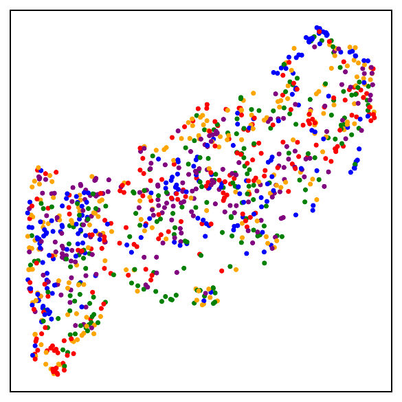
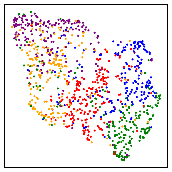
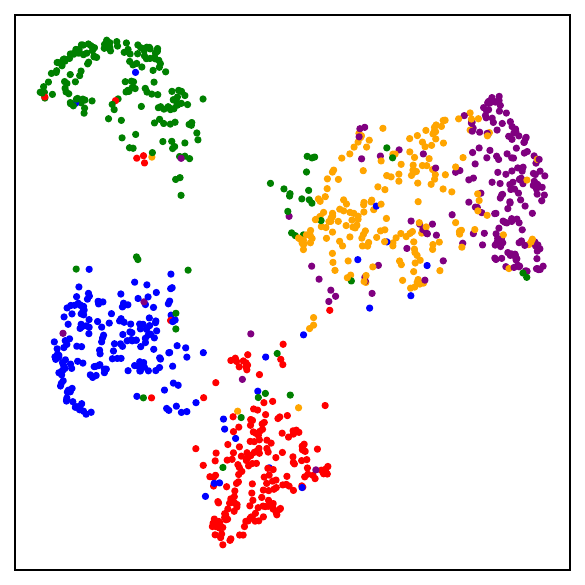
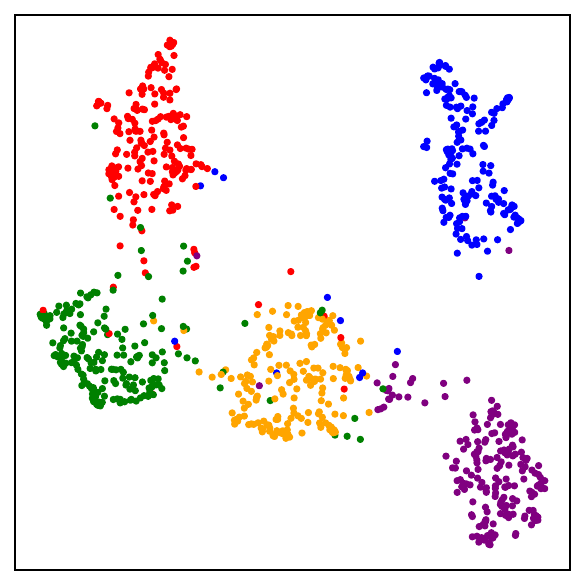
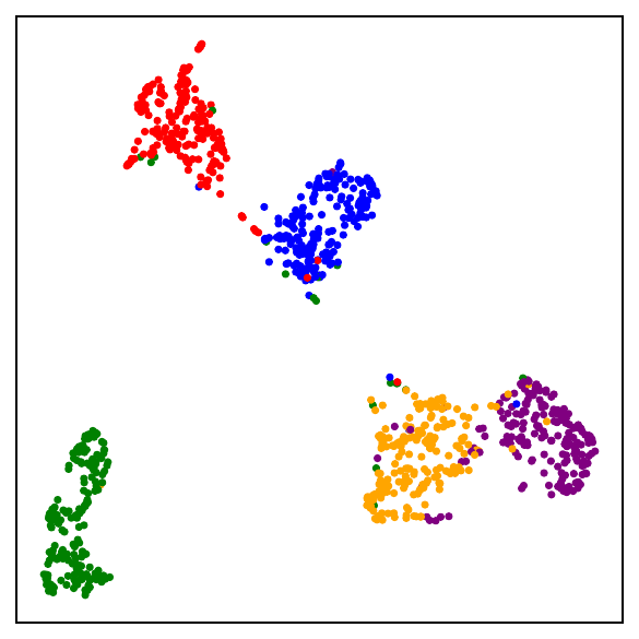
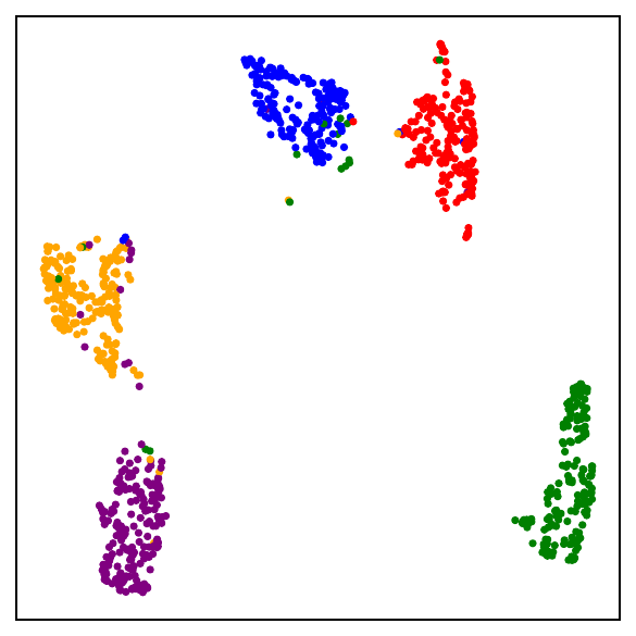
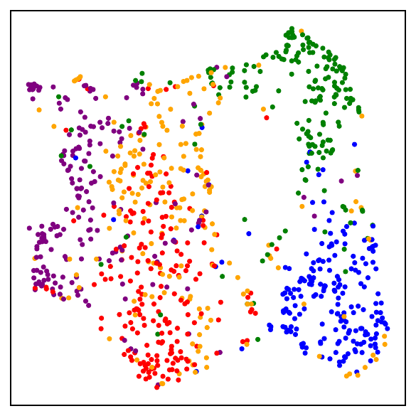
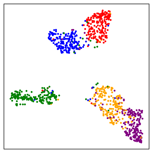
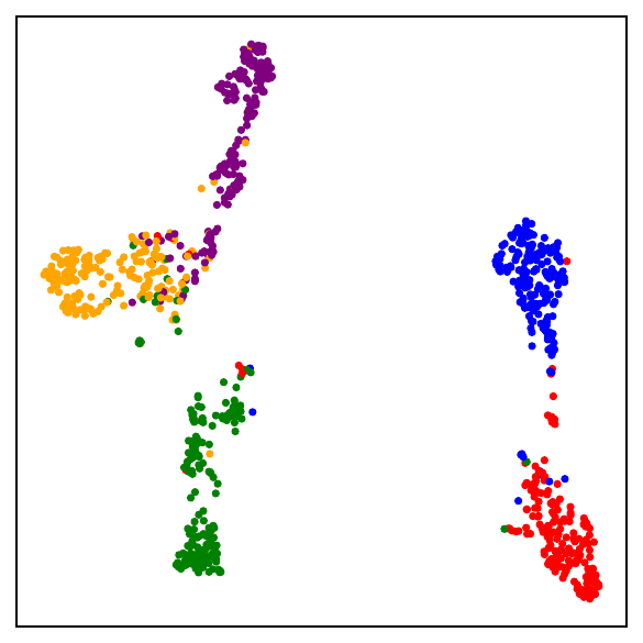
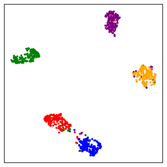
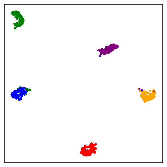
Fig. 1. UMAP visualizations on mini-ImageNet across training. DCL (self-supervised, top) progressively forms semantic clusters without access to labels. NSCL (supervised, bottom) yields tighter clusters. Both runs start from the same random initialization.
Part I — A supervised objective sits very near the self-supervised one
The setup
Consider a labeled dataset $S = \{(x_i, y_i)\}_{i=1}^N$, but suppose that during self-supervised training we only use the inputs $x_i$, not the labels. For each sample $x_i$, we generate $K$ augmentations and map them through an encoder $f$. A standard decoupled contrastive loss (DCL) takes the form:
Compare it with the negatives-only supervised contrastive learning (NSCL) variant:
The numerator and positive pairs are identical. The only difference is in the denominator:
Why the gap is small
Fix an anchor. In DCL, the denominator sums over all $N-1$ other samples. In NSCL, it sums over only the $N - n = n(C-1)$ different-class samples. The discrepancy is controlled by a simple quantity: the fraction of the denominator occupied by same-class samples. In a balanced $C$-class problem, that fraction is roughly $1/C$.
This can be made precise:
The bound holds for any encoder $f$, without assumptions on data distribution or model class. For problems with many semantic classes, DCL is already very close to NSCL.
Validating the bound during training
Training models using SimCLR to minimize the DCL loss, tracking both losses throughout training alongside the theoretical upper bound, confirms that all three quantities are highly correlated — and that the gap tightens as $C$ grows.
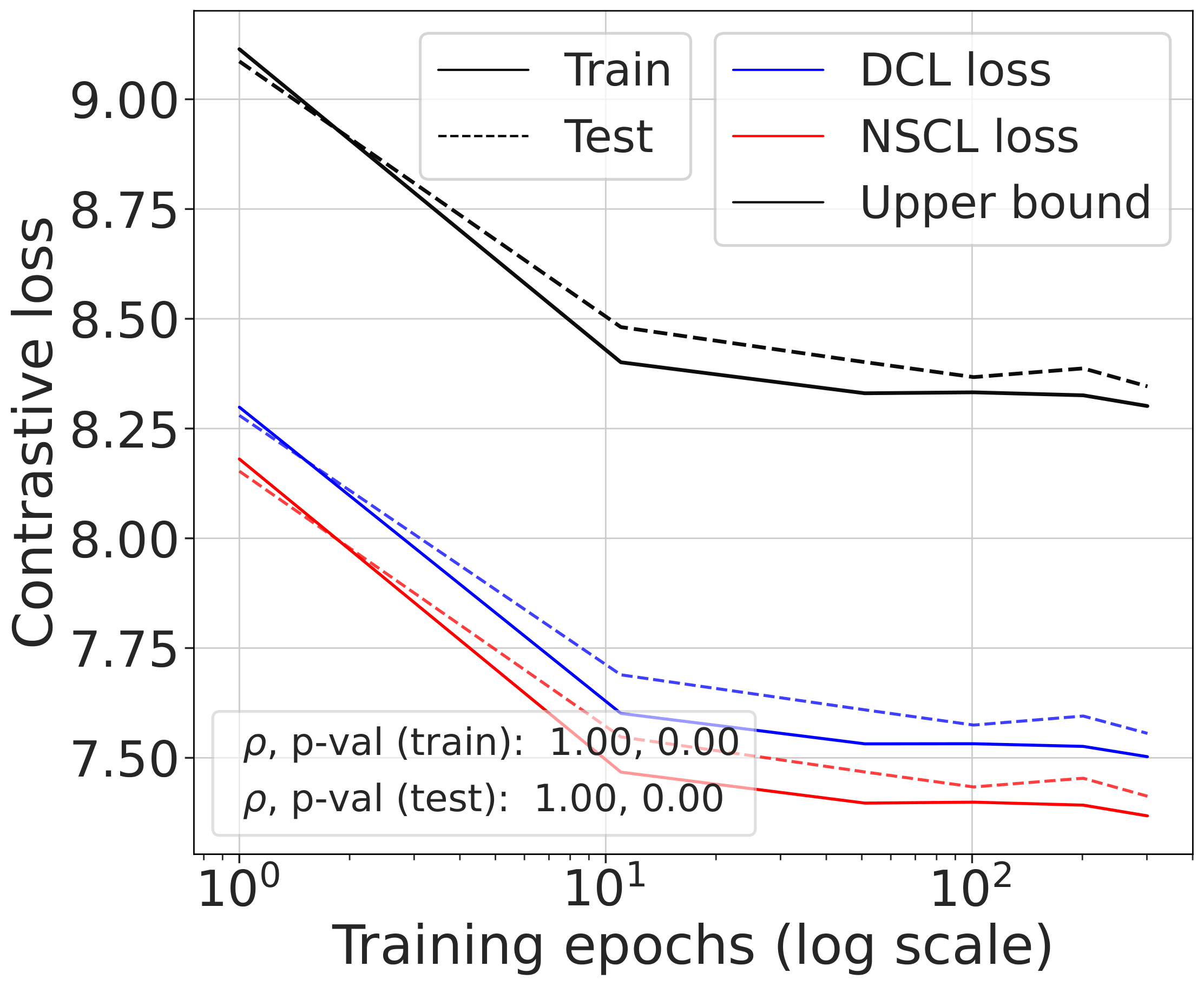
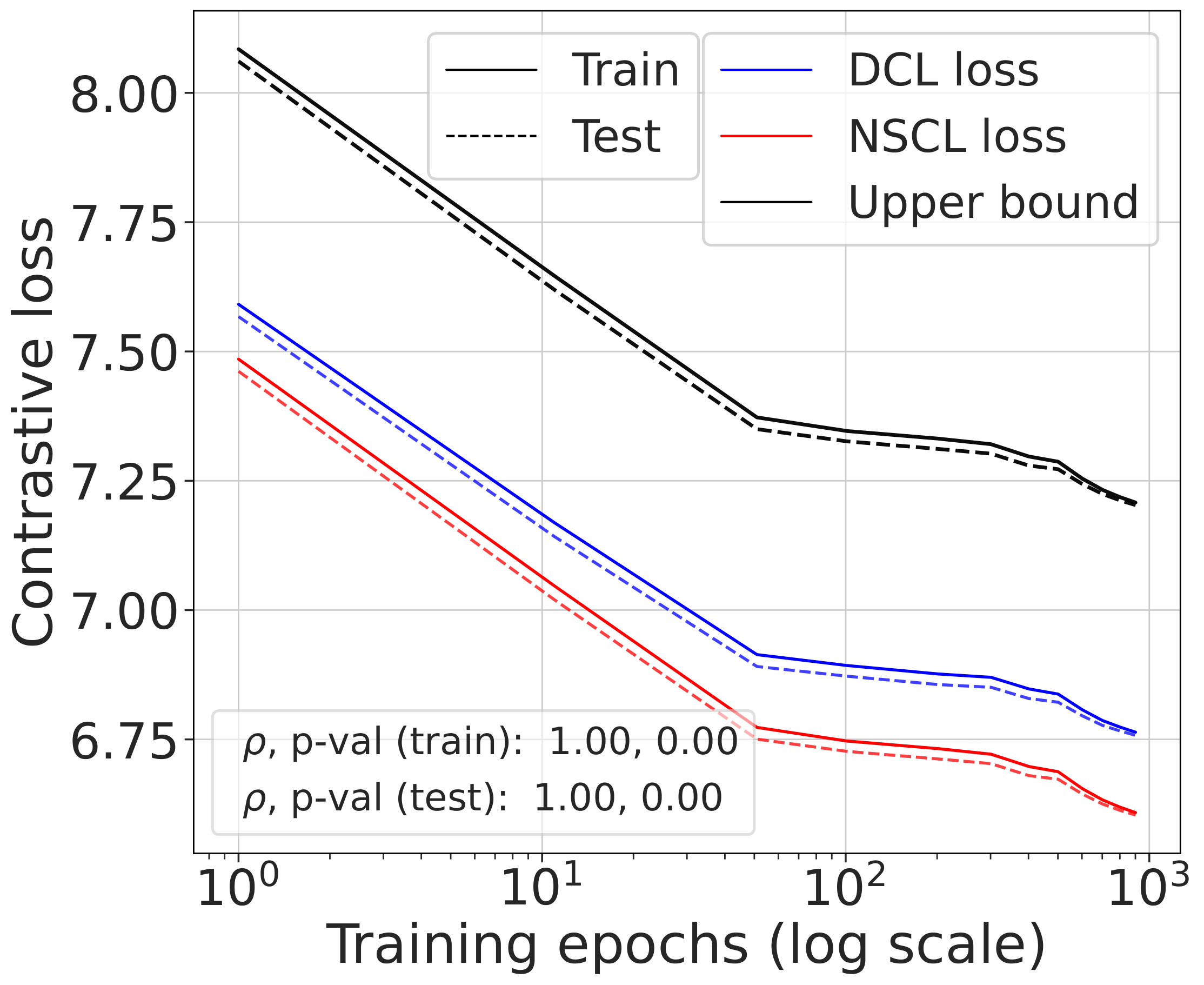
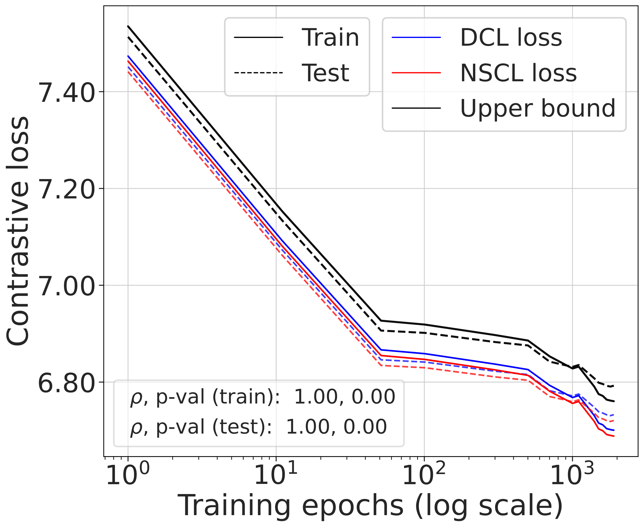
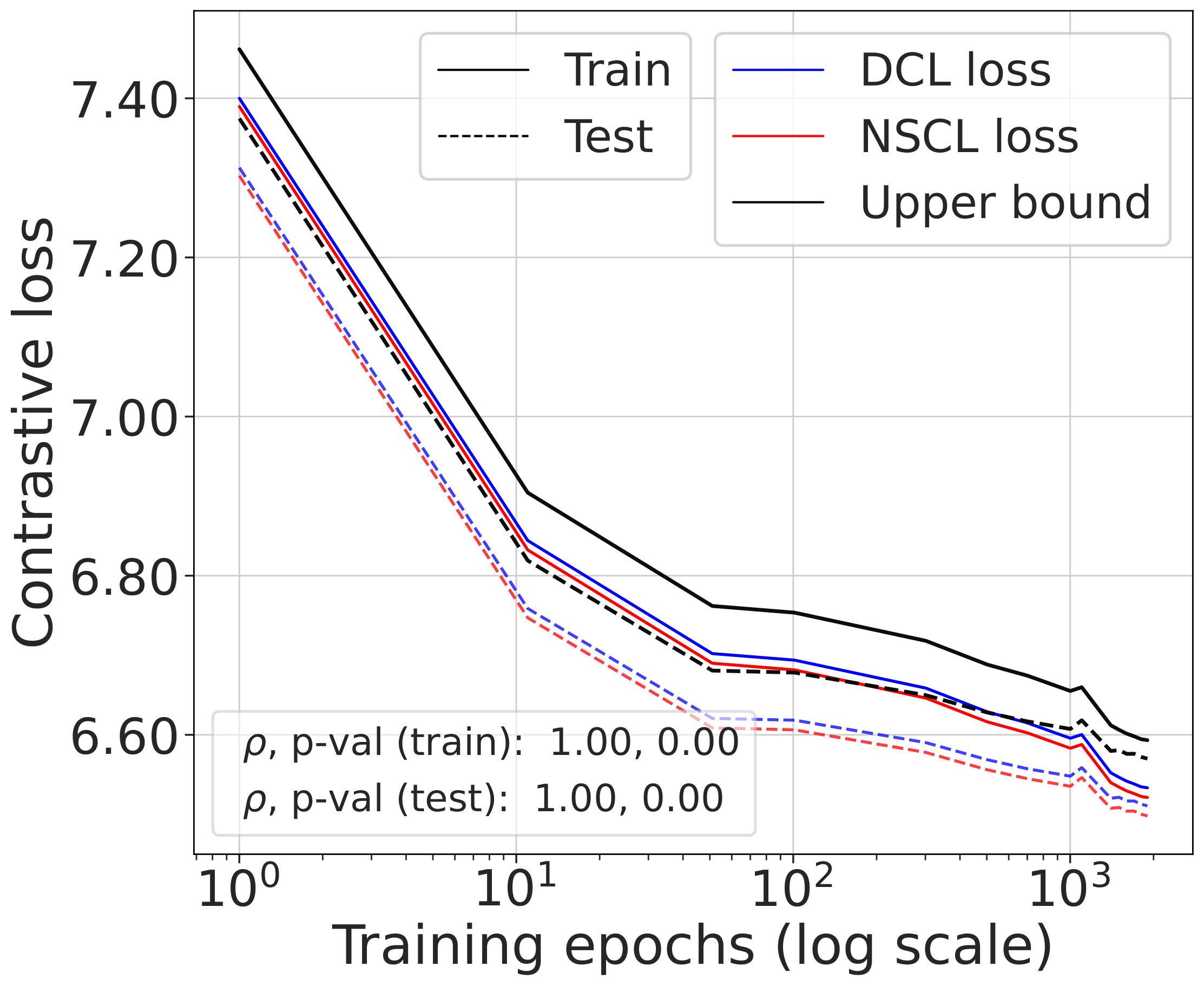
Fig. 2 (top). DCL loss, NSCL loss, and the theoretical bound tracked during SimCLR training. All three quantities are highly correlated. The gap between DCL and NSCL becomes tighter as the number of classes increases; compare CIFAR-10 with CIFAR-100.
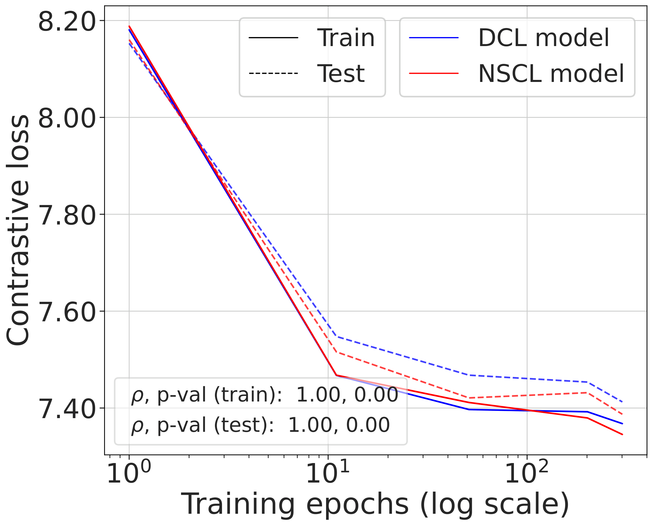
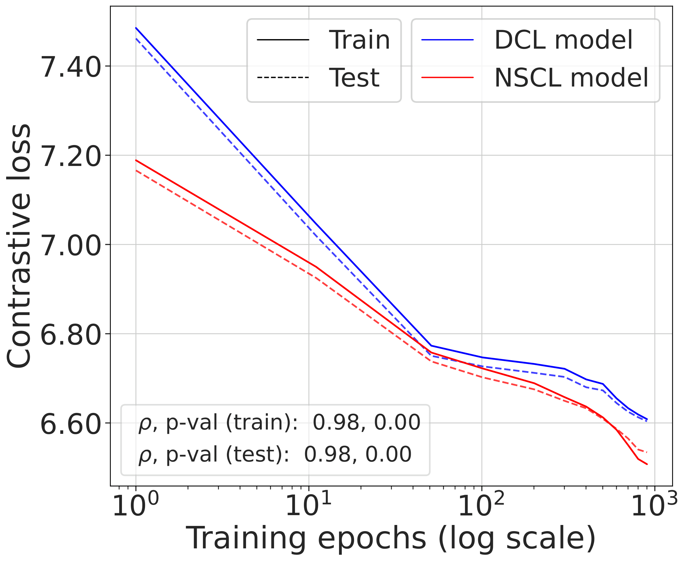
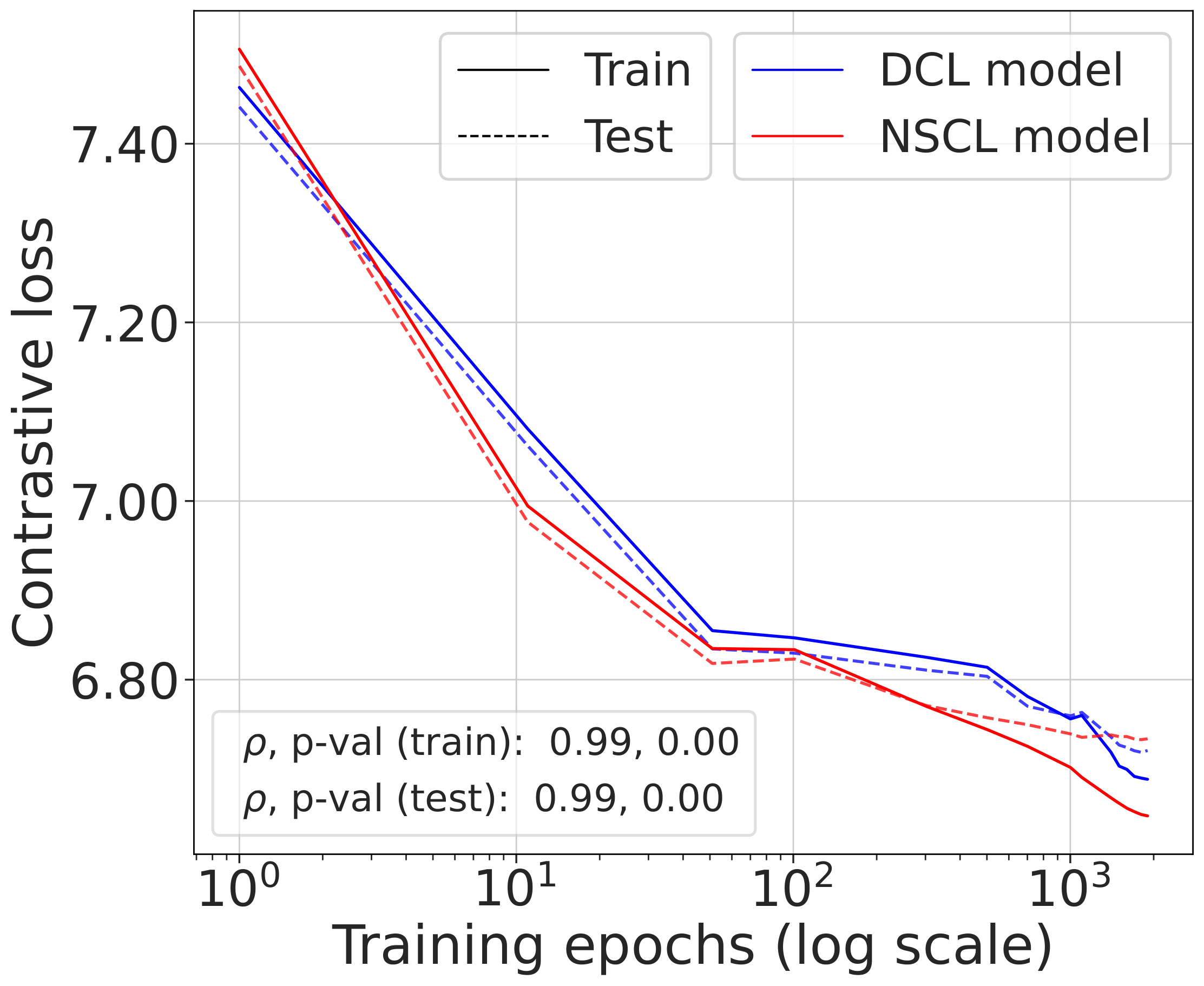
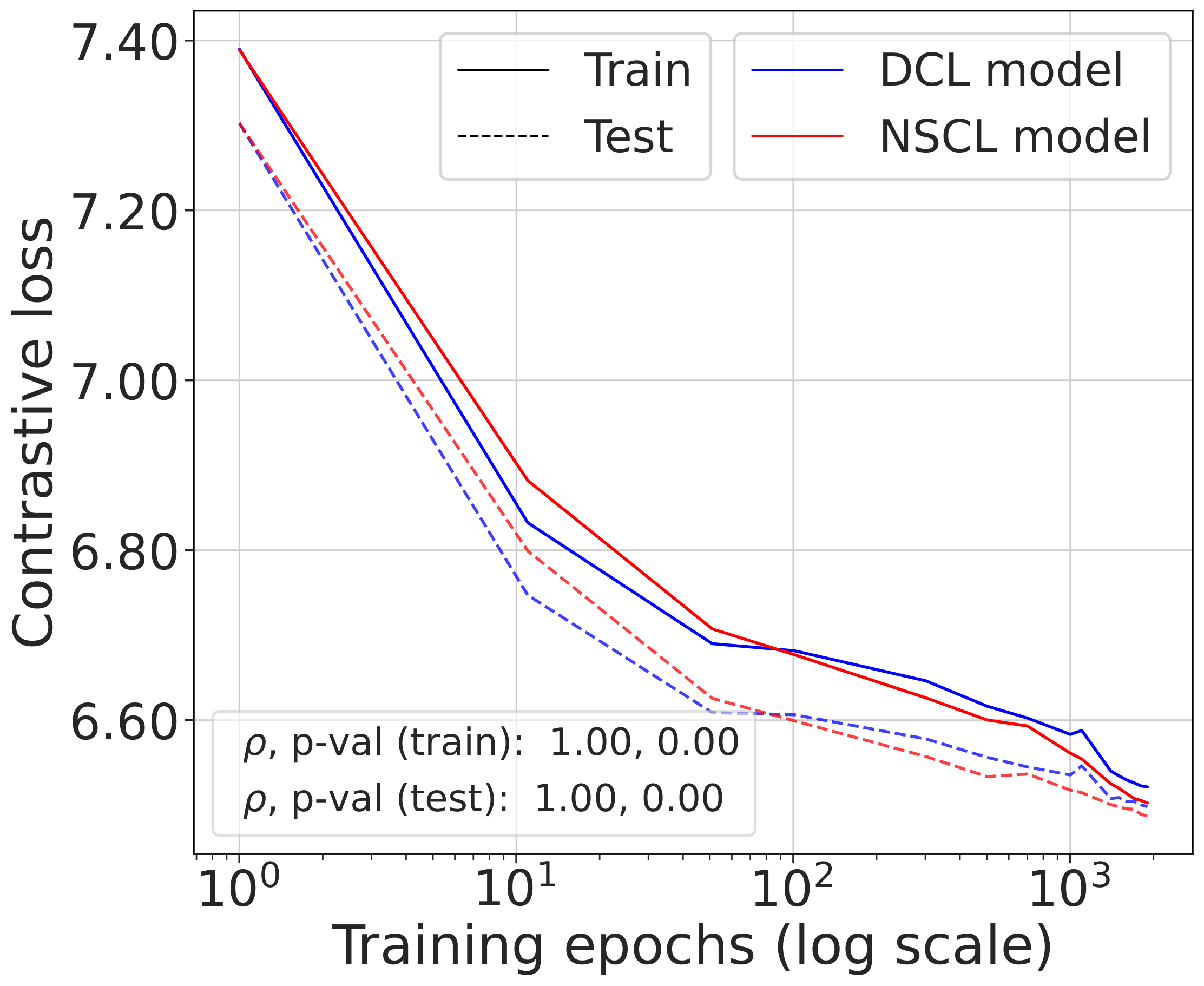
Fig. 2 (bottom). Comparing the NSCL loss of two models — one trained with DCL, one with NSCL. The resulting NSCL losses are comparable regardless of training objective, suggesting minimizing DCL already brings the NSCL loss close to the value achieved by direct NSCL minimization.
The gap scales as predicted with $C$
The gap $\mathcal{L}^{\text{DCL}} - \mathcal{L}^{\text{NSCL}}$ as a function of the number of classes $C$ follows the theoretical bound $\log(1 + e^2/(C-1))$ closely across all training epochs and datasets.
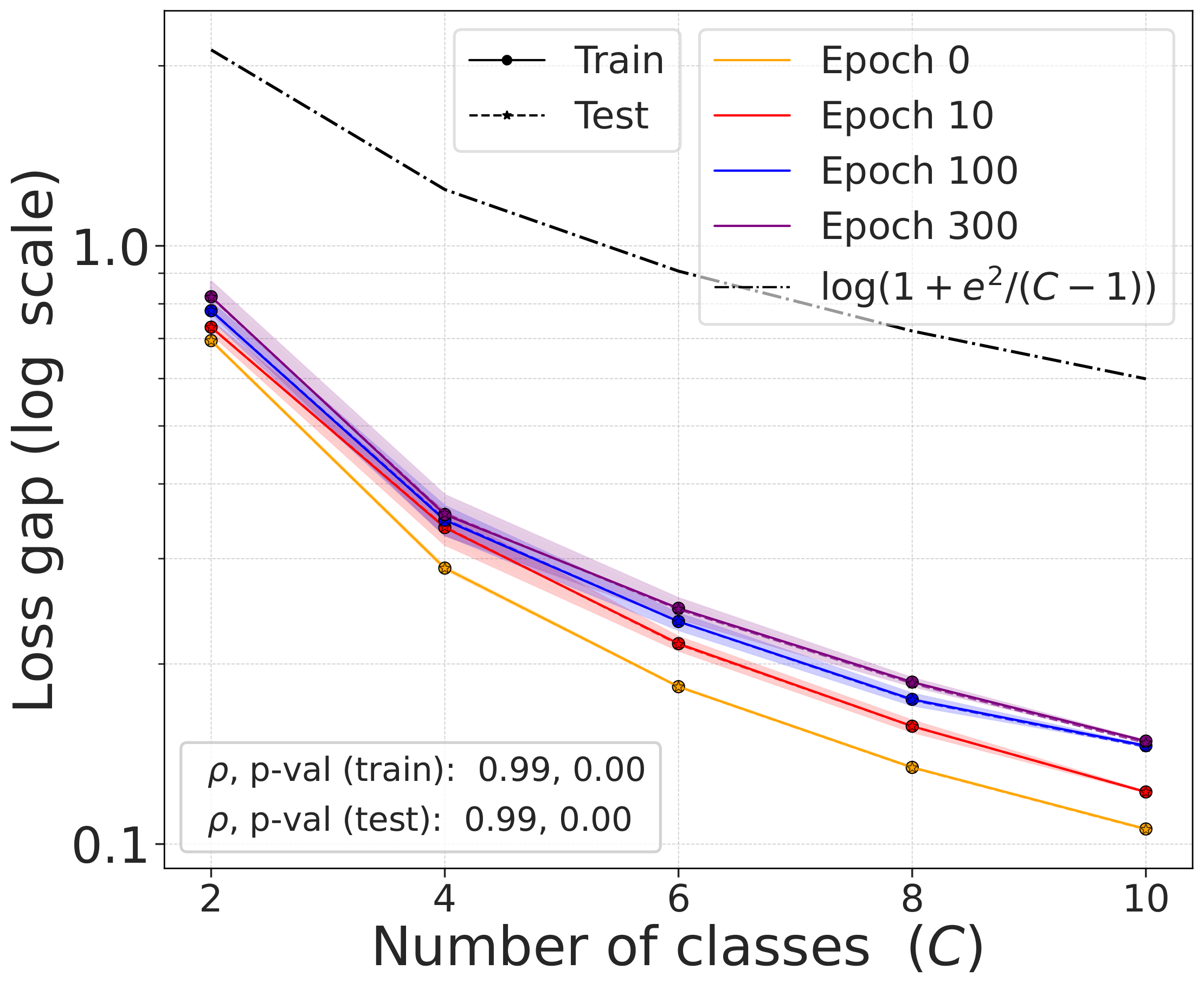
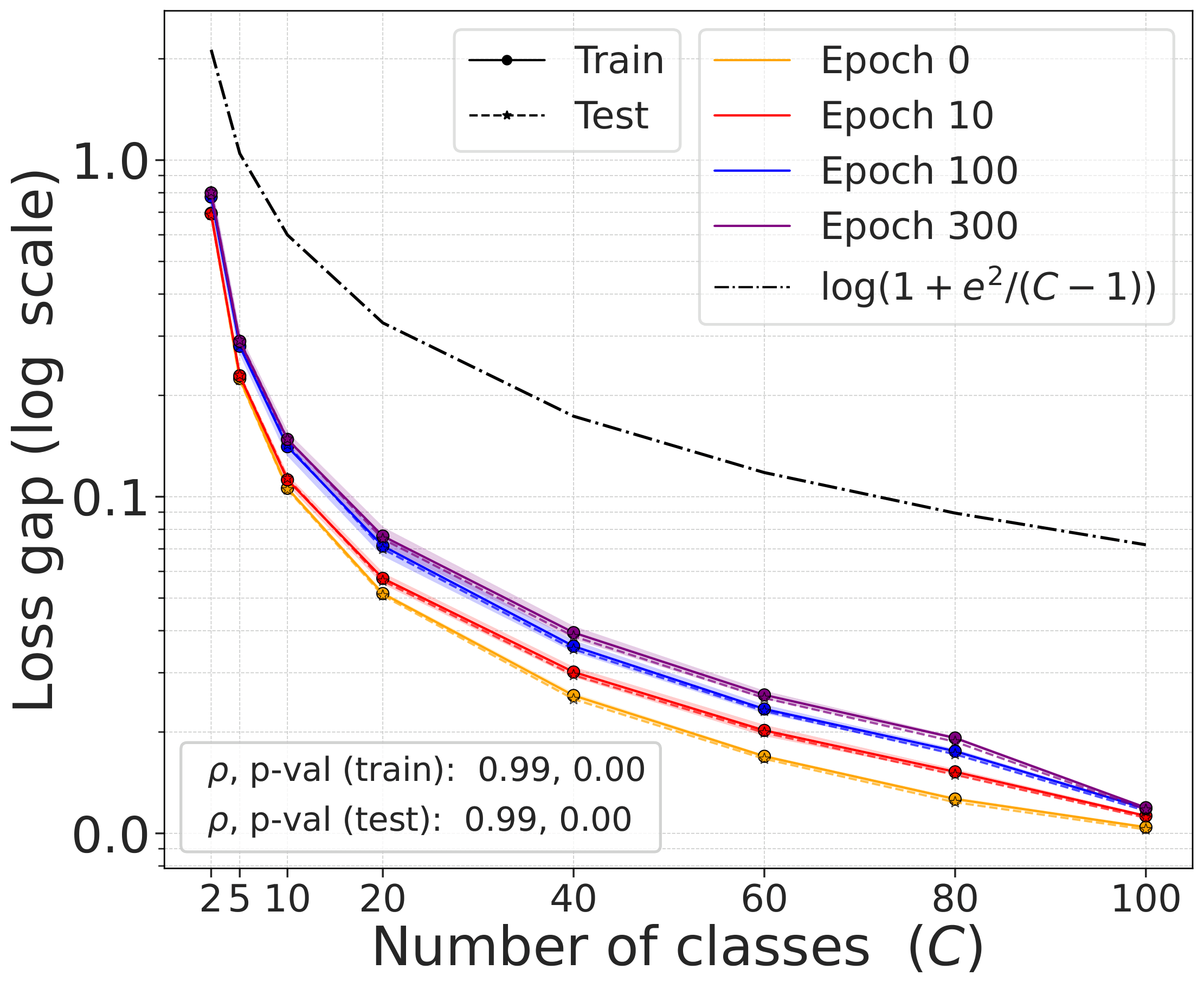
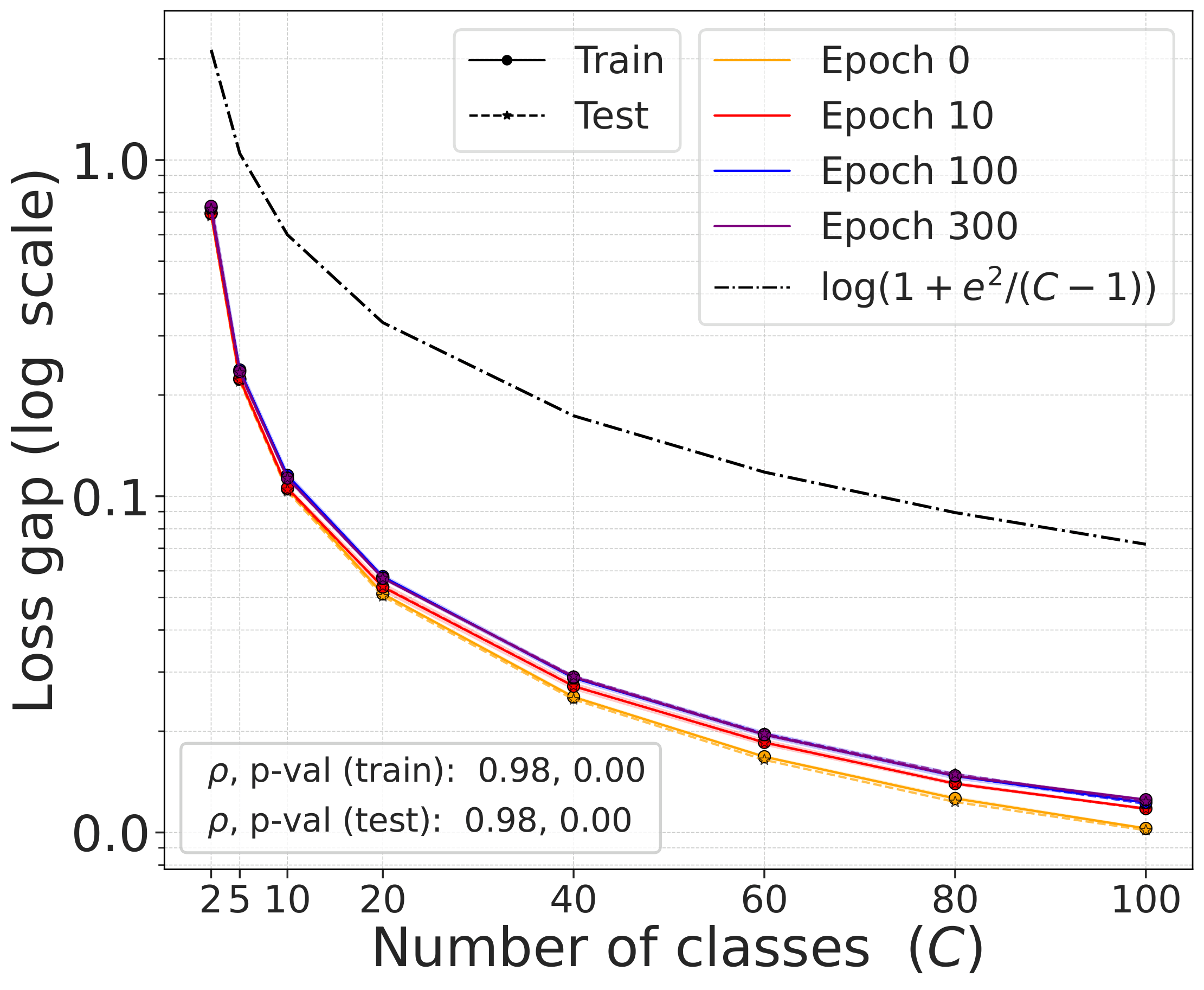
Fig. 3. The gap $\mathcal{L}^{\text{DCL}} - \mathcal{L}^{\text{NSCL}}$ as a function of $C$, compared with the theoretical bound. The gap shrinks with $C$ at all training epochs.
What NSCL minimizers look like
Since DCL sits close to NSCL at the level of the loss, it is natural to ask what the global minimizers of NSCL look like. The answer is remarkably structured:
This places NSCL within the same broader geometric picture that appears in supervised learning. The supervised problem adjacent to DCL is not arbitrary; it has the same neural-collapse structure familiar from other well-studied supervised objectives.
Part II — The learned representations stay close
Loss-level closeness is informative, but it does not by itself imply similar learned geometry. Two nearby objectives can still drive optimization in meaningfully different directions. The second paper addresses this directly.
Shared-randomness coupling
Consider training DCL and NSCL under shared randomness: same initialization, same mini-batches, same augmentations, same hyperparameters. The only difference is the objective. The cosine similarity matrix $\Sigma(Z)_{ij} = \cos(z_i, z_j)$ provides the basis for CKA and RSA comparison.
The similarity matrices stay close
Under this coupled training protocol, the difference between DCL and NSCL similarity matrices satisfies:
The right-hand side becomes smaller when $C$ is larger, $B$ is larger, $\tau$ is higher, and cumulative step size is moderate. This immediately yields lower bounds on CKA and RSA:
Empirical confirmation
DCL and NSCL models trained under exactly matched conditions for 300 epochs yield consistently high alignment scores:
Fig. 5. Representation similarity between DCL and NSCL models trained with matched initialization and mini-batch order. All values exceed 0.81. Alignment is strongest when the number of classes is largest (CIFAR-100, mini-ImageNet), matching the theory. Scores are nearly identical across ResNet-50 and ViT-Base.
Two patterns are especially notable. First, alignment is strongest when the number of classes is largest — CIFAR-100 and mini-ImageNet reach 0.91+ — matching the theory that more classes imply a smaller loss gap. Second, scores are nearly identical across ResNet-50 and ViT-Base, indicating the DCL-NSCL relationship is not an artifact of a particular architecture.
But weights can still diverge
In contrast, parameter-space coupling is much less stable. The weight-space bound has no batch-size moderation in the exponent, so representation-level alignment can remain stable even when parameter-space divergence becomes large.
The right mental model
The standard description is that contrastive learning is a self-supervised method that nonetheless learns semantic structure. While true, it leaves open why this happens so consistently.
The picture here is more specific. The self-supervised contrastive objective is already close to a supervised contrastive objective that excludes same-class negatives. That supervised objective has global minimizers with the same neural-collapse geometry familiar from supervised learning. And under shared training randomness, the two methods learn highly aligned representations throughout training.
This does not mean that self-supervised and supervised learning are identical, nor that labels are irrelevant. But it does suggest that the gap between the two is narrower, and more structured, than the usual informal description implies.
Takeaway
The main point is not merely that self-supervised and supervised contrastive learning are related. It is that the relation is surprisingly tight and structurally clean.
The objectives are close. The standard self-supervised contrastive loss approximates the NSCL loss, with a gap that shrinks as $O(1/C)$.
The nearby supervised problem has elegant geometry. NSCL minimizers exhibit augmentation collapse, within-class collapse, and simplex ETF structure.
The learned representations stay aligned. Under shared training randomness, DCL and NSCL produce highly similar representation geometry (CKA, RSA > 0.81), even when their parameters diverge.
A useful way to view contrastive learning, then, is not as a completely separate mechanism that somehow recovers semantics, but as a self-supervised procedure whose objective and learned geometry already lie close to a specific supervised counterpart.
Comments